A 209M Model Beat Larger Forecasting AIs? What Mistral Hasn't Proven

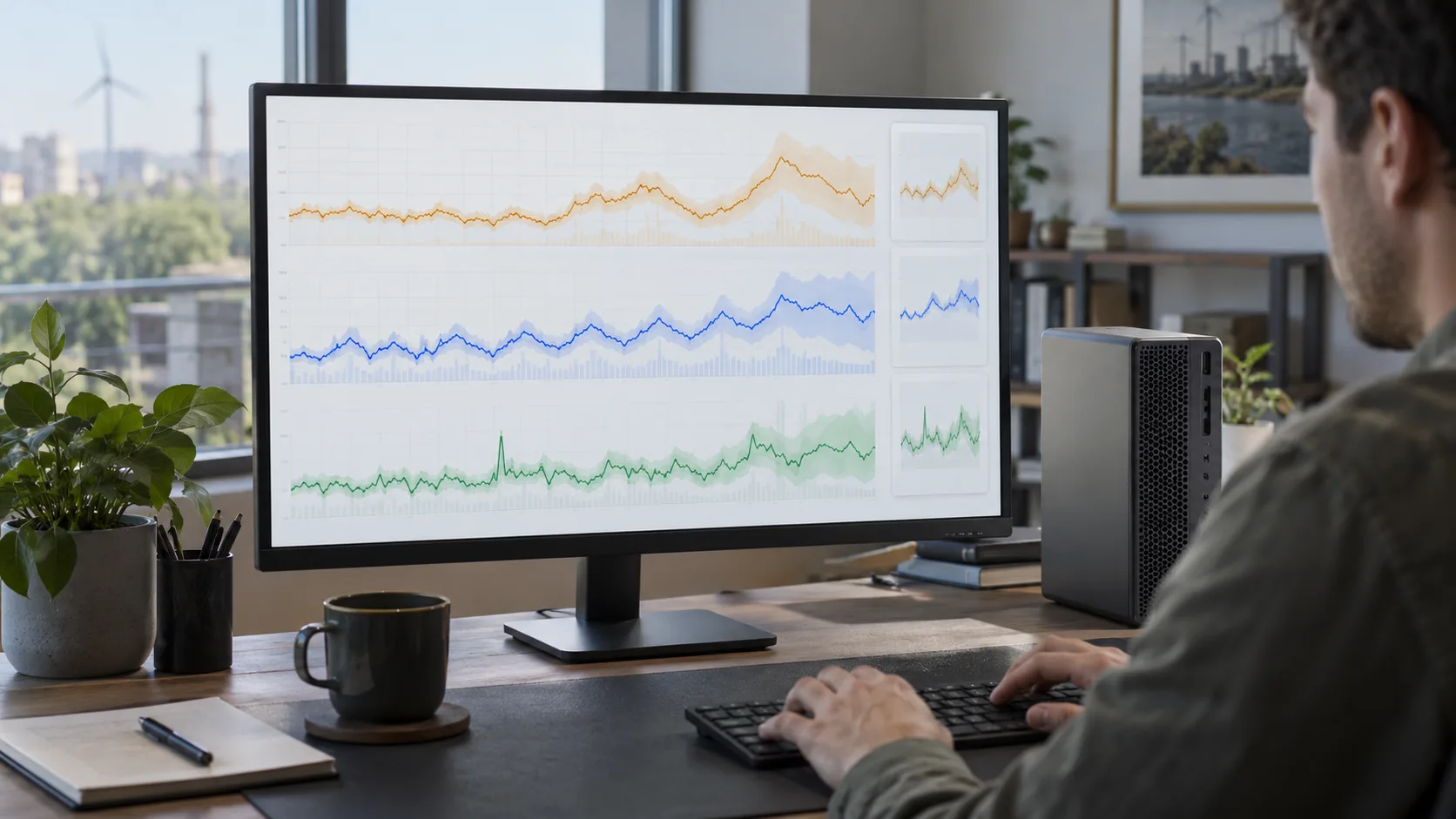
Mistral says its 209-million-parameter Timestral model ranks first among pretrained zero-shot systems on three public forecasting benchmarks, beating models with far more parameters while running on a CPU. The result is notable, but it does not prove that Timestral will beat every larger forecasting model on a company’s real data. The full technical report is still forthcoming, and the launch comparisons cover a defined benchmark class.

That distinction matters because leaderboard announcements tend to travel faster than the caveats attached to them. A reader who sees “209M beats much larger models” may reasonably conclude that scale no longer matters in forecasting. The more careful reading is that scale is not the only lever, and that a benchmark class defined by zero-shot evaluation rewards different qualities than a production deployment does. Mistral’s own framing keeps the claim inside that class; the surrounding context is what determines whether the claim travels well.

Timestral is not a chatbot. It is a family of time-series foundation models designed to forecast numerical sequences such as energy demand, inventory, sensor readings, cash flow, capacity, or equipment behavior. The family comes in 5M, 28M, 123M, and 209M sizes.

The spread of sizes is itself part of the pitch. A team with a modest observability stack and a few dozen server metrics does not need the largest checkpoint, and a team forecasting thousands of related retail series may want the headroom. Offering the family in four sizes signals that Mistral expects deployment to vary by latency budget, hardware, and accuracy requirement rather than converging on one configuration.

What the benchmark claim means

Mistral reports that Timestral-209M ranks first among pretrained and zero-shot entries on GIFT-Eval, TIME, and fev-bench. Zero-shot means the checkpoint is evaluated without retraining it specifically for each target dataset. That matters because many older forecasting systems must be fitted separately to every series or organization.

Fitting separately is expensive in ways that rarely show up in accuracy tables. Each series needs its own configuration, validation split, and maintenance path, and a change in the underlying process can silently invalidate a fitted model. Zero-shot evaluation asks a different question: how well does one checkpoint generalize across datasets it has never been tuned on? A strong answer there suggests lower marginal cost for each new series a team wants to forecast, even if a tuned model could beat it on any single well-understood series.

According to the published model card, Timestral supports univariate and multivariate forecasts, past-only and known-future covariates, and probabilistic outputs across 21 quantiles. It can use up to 32,768 historical steps and predict up to 1,024 steps in a single forward pass.

Those capabilities fit real planning problems better than a single best-guess line. A power operator may know tomorrow’s weather, a factory may know its production schedule, and a retailer may know holidays. Timestral can incorporate such known-future variables while producing a distribution rather than pretending that one exact number is certain.

The 21-quantile output is the detail most likely to be undervalued by readers who focus on the ranking. Planning systems rarely consume a point forecast in isolation; they consume a range to size buffers, staff shifts, or safety stock. A model that emits a distribution in one pass removes a layer of downstream machinery, though it also raises a new question: whether those quantiles stay honest when the world shifts. That question is answered by backtesting, not by a benchmark score.

The context window deserves similar scrutiny. Thirty-two thousand historical steps is generous for daily series and modest for high-frequency sensor data, where a single day of 15-minute observations is already 96 steps. The practical meaning depends on sampling frequency, and the model card’s limits should be read against a team’s actual cadence rather than treated as a universal capacity.

How a small model can beat a larger one

Parameter count is not a universal measure of forecasting quality. A specialized architecture trained for numerical sequences can outperform a bigger general model on a narrow task. Timestral uses patch-based processing, attention across time and variables, and a forecasting design that preserves historical context while generating future blocks.

Patch-based processing is the mechanism worth understanding. Rather than treating each timestamp as an isolated token, the model groups consecutive observations into patches, which changes the effective sequence length and lets attention operate over coarser units. Combined with attention across variables, this lets the model represent relationships between signals that move together, such as pressure and temperature, without hand-engineering those relationships. A general-purpose language model has no particular reason to represent such structure efficiently; a model built for numerical sequences does.

Mistral also says most pretraining data was synthetic, followed by post-training on a mixture of real and synthetic series. This can expose the model to varied trends, seasonal patterns, noise, missing data, and cross-variable relationships without depending entirely on scarce proprietary datasets.

Synthetic pretraining is a deliberate trade. Real forecasting corpora are fragmented, inconsistently formatted, and often proprietary, so a model that relied on them alone would inherit their gaps. Generating varied series lets the designers control the mix of trends, seasonality, noise, and missingness the model sees. The cost is a distribution gap between synthetic and real data, which is precisely why the post-training mixture includes real series and why independent evaluation on production data remains the decisive test.

The result is efficiency. Mistral reports that the 209M model can forecast one day from three weeks of 15-minute observations in about 140 milliseconds on a standard eight-thread server CPU. The smallest 5M model reportedly does the same class of task in about 10 milliseconds.

Those numbers reframe the deployment conversation. A forecast that completes in 140 milliseconds on commodity hardware can run inside a request path, not only in a nightly batch. The 10-millisecond variant makes high-frequency scoring plausible on the same servers that already handle the data pipeline, which changes the economics of testing several models side by side.

What remains unverified

First, the benchmark framing is narrower than “best forecasting AI.” The rankings apply to pretrained, zero-shot models under specified evaluation rules. A domain-specific model trained on a company’s own history may perform better. Classical systems such as ARIMA or gradient-boosted models can also remain competitive when data is stable, limited, or strongly understood.

That is not a rhetorical hedge. Benchmark suites aggregate across datasets with different frequencies, horizons, and difficulty, and an average rank can hide losses on the specific series a team cares about. A retailer with stable weekly seasonality may find a tuned classical model cheaper and more predictable to operate. A team with hundreds of short, noisy series may find the opposite. The benchmark tells you where to look; it does not tell you what you will find.

Second, Mistral has published code, checkpoints, and score tables, but says a full technical report will follow. Independent teams still need to reproduce the results, inspect data overlap risks, and test whether the model’s uncertainty estimates remain calibrated under distribution shifts.

Data overlap is the quiet risk in any foundation-model claim. If evaluation series resemble pretraining series too closely, zero-shot scores can flatter the model without reflecting genuine generalization. Reproduction by outside teams, with attention to how evaluation windows were constructed, is the standard remedy. Calibration under distribution shift is the second open question: a model can rank well on point error while its quantiles drift, which matters more to anyone sizing a buffer than to anyone reading a leaderboard.

Third, the Modified MIT license on model weights is not identical to the Apache 2.0 license covering the repository code. Commercial teams should read the weight license instead of assuming the package and checkpoint share the same terms.

This is a small point with outsized consequences. Engineers typically encounter the repository first and infer licensing from it; legal review happens later, sometimes after a prototype has already shaped a roadmap. Treating the weight license as a separate document to be read before adoption avoids that sequence.

Where Timestral could be useful

The strongest immediate use cases are environments with many related series: industrial sensors, server observability, energy loads, retail demand, financial flows, and maintenance signals. Multivariate forecasting can capture relationships between pressure, vibration, and temperature instead of treating every signal independently.

CPU inference also lowers deployment friction. A team can test the model on premises or in an air-gapped network without provisioning a GPU cluster. The 837MB full-precision 209M checkpoint is small enough for ordinary servers, and smaller variants offer lower latency when accuracy requirements permit it.

Air-gapped operation is easy to overlook until it is the binding constraint. Organizations in utilities, manufacturing, and regulated finance often cannot route telemetry through an external service, and a checkpoint that fits on an ordinary server removes a procurement conversation from the critical path. The same property makes local experimentation cheap: a team can compare Timestral against its incumbent without committing to new infrastructure.

Still, deployment should begin as a shadow forecast. Run Timestral beside the existing model, record errors by horizon and regime, test rare events, and verify that uncertainty bands correspond to actual outcomes. Replacing a planning system solely because of a leaderboard would repeat the mistake that the small-model story is supposed to challenge.

A shadow period also produces the evidence a benchmark cannot: how the model behaves on the team’s own holidays, outages, promotions, and structural breaks. Recording errors by horizon and regime turns a vague impression into a comparison, and checking whether the quantile bands match realized outcomes tests the calibration claim directly. Rare events deserve separate attention because they are where planning failures concentrate and where aggregate scores are least informative.

Verdict

Timestral makes a strong case that architecture, data, and task fit matter more than raw model size. A 209M forecasting model leading three public zero-shot benchmarks and running on CPUs is genuinely useful progress.

The missing piece is broad independent validation on messy production data. The right headline is not “small AI defeats every large model.” It is that specialized, open-weight forecasting has become cheap enough to test almost anywhere—and the burden now shifts to operators to prove that the public benchmark advantage survives contact with their own data.

For readers, that shift is the actionable part. The cost of finding out whether Timestral fits a given workload has fallen to a checkpoint download and a shadow run, and the questions worth asking are concrete: does it hold up on our series, are its quantiles calibrated through our disruptions, and do the weight terms permit the use we intend? Those are answerable without waiting for the technical report, even though the report will sharpen the answers.